시계열 데이터
시계열 데이터는 데이터 분석 분야에서 중요하게 다루는 데이터 중 하나이다. 일정 시간 간격으로 어떤 값을 기록한 데이터에서 시계열 데이터가 매우 중요하다.
Datetime 오브젝트
datetime 라이브러리는 날짜와 시간을 처리하는 등의 다양한 기능을 제공하는 파이썬 라이브러리이다.
datetime 라이브러리에는 날짜를 처리하는 date 오브젝트, 시간을 처리하는 time 오브젝트, 날짜와 시간 모두 처리하는 datetime 오브젝트가 포함되어 있다.
from datetime import datetime

now1 = datetime.now()
print(now1)

now2 = datetime.today()
print(now2)
now, today 메서드를 사용하면 현재 시간을 출력할 수 있다.
또한 datetime 오브젝트를 생성할 때 시간을 직접 입력하여 전달할 수 있다.
t1 = datetime(1970, 1, 1)
print(t1)
datetime 오브젝트를 사용하는 이유 중 하나는 시간 계산을 할 수 있다는 점이다.
t1 = datetime(1970, 1, 1)
t2 = datetime(1970, 12, 12, 13, 24, 34)
diff1 = t1 - t2
print(diff1)
print(type(diff1))
경우에 따라서는 시계열 데이터를 문자열로 저장해야 할 때도 있다. 이럴 때는 to_datetime 메서드를 사용하여 datetime 오브젝트로 변환해 주어야 한다.
import pandas as pd
import os

ebola = pd.read_csv('../data/country_timeseries.csv')
print(ebola.info())
Date가 object로 설정되어 있는 것을 볼 수 있다. 이를 to_datetime 메서드로 datetime 오브젝트로 변환해보자.
ebola['date_df'] =pd.to_datetime(ebola['Date'])
print(ebola.info())
date_df는 Dtype이 datetime이라는 것을 확인할 수 있다.
to_datetime 메서드는 시간 형식 지정자(%d, %m, %y)와 기호(/, -)를 적절히 조합하여 fomat 인자에 전달하면 형식을 지정할 수 있다.
test_df1 = pd.DataFrame({'order_day':['01/01/15', '02/01/15', '03/01/15']})

test_df1['date_dt1'] = pd.to_datetime(test_df1['order_day'], format='%d/%m/%y')
test_df1['date_dt2'] = pd.to_datetime(test_df1['order_day'], format='%m/%d/%y')
test_df1['date_dt3'] = pd.to_datetime(test_df1['order_day'], format='%y/%m/%d')

print(test_df1)
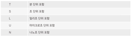
형식 지정자는 다음과 같다.
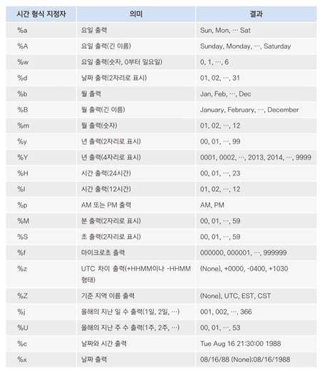

strfrime 메서드와 시간 형식 지정자를 이용하면 원하는 형식의 datetime을 쉽게 얻을 수 있다.
now = datetime.now()
print(now)

nowDate = now.strftime('%Y-%m-%d')
print(nowDate)
read_csv 메서드의 parse_dates 인자에 datetime 오브젝트로 변환하고자 하는 열의 이름을 전달하여 데이터 집합을 불러오면 쉽게 datetime 오브젝트로 변환할 수 있다.
ebola1 = pd.read_csv('../data/country_timeseries.csv', parse_dates=['Date'])
print(ebola1.info())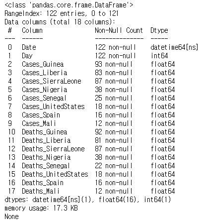
Date열이 datetime 오브젝트인 것을 알 수 있다.
datetime 오브젝트의 year, month, day 속성을 이용하여 년, 월, 일 정보를 따로 추출할 수 있다.
date_series = pd.Series(['2018-05-16', '2018-05-17', '2018-05-18'])
d1 = pd.to_datetime(date_series)
print(d1)
print(d1[0].year)
print(d1[0].month)
print(d1[0].day)
dt 접근자
문자열을 처리하려면 str 접근자를 사용하는 것과 마찬가지로 datetime 오브젝트에 접근하려면 dt 접근자를 사용할 수 있다.
ebola = pd.read_csv('../data/country_timeseries.csv')
ebola['date_dt'] = pd.to_datetime(ebola['Date'])

ebola['year'] = ebola['date_dt'].dt.year
print(ebola[['Date', 'date_dt', 'year']].head())

이 열의 dtype은 int이다.
시계열 데이터 계산
ebola 데이터프레임으로 시계열 데이터를 어떻게 계산하는지 살펴보자.
print(ebola.iloc[-5:, :5])
print(ebola['date_dt'].min())
print(type(ebola['date_dt'].min()))
최초 발병일을 알아냈다. Date 열에서 최초 발병일을 빼 진행 정도를 알아보자.
ebola['outbreak_d'] = ebola['date_dt'] - ebola['date_dt'].min()
print(ebola[['Date', 'Day', 'outbreak_d']].head())
파산한 은행의 개수를 계산해보자.
banks = pd.read_csv('../data/banklist.csv')
print(banks.head())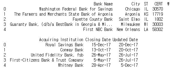
Closing Date, Update Date의 자료형은 문자열이기 때문에 이를 시계열 데이터로 로드해보자.
banks = pd.read_csv('../data/banklist.csv', parse_dates=['Closing Date', 'Updated Date'])
print(banks.info())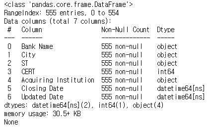
dt 접근자와 quarter 속성을 이용하면 은행이 파산한 분기를 알 수 있다.
banks['closing_quarter'], banks['closing_year'] = (banks['Closing Date'].dt.quarter, banks['Closing Date'].dt.year)
print(banks.head())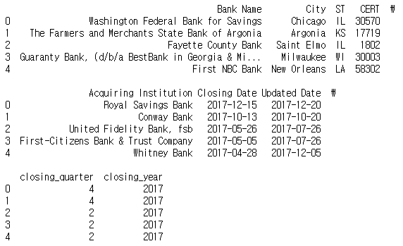
closing_year = banks.groupby(['closing_year']).size()
print(closing_year)
closing_year_q = banks.groupby(['closing_year', 'closing_quarter']).size()
print(closing_year_q)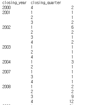
import matplotlib.pyplot as plt

fig, ax = plt.subplots()

ax = closing_year.plot()
plt.show()

fig, ax = plt.subplots()

ax = closing_year_q.plot()
plt.show()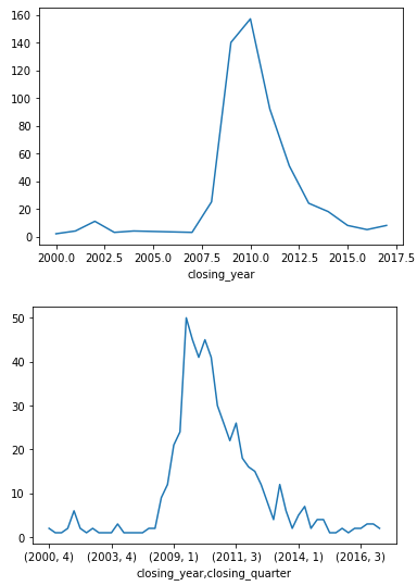
datetime 오브젝트와 인덱스
datetime 오브젝트를 데이터프레임의 인덱스로 설정하면 원하는 시간의 데이터를 바로 추출할 수 있어 편리하다.
banks.index = banks['Closing Date']
print(banks.index)
banks = banks.sort_index()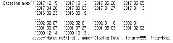
datetime 오브젝트를 인덱스로 지정하면 다음과 같은 방법으로 원하는 시간의 데이터를 바로 추출할 수 있다.
print(banks['2015'].iloc[:5, :5])
2015년의 데이터를 추출한 것이다.
시간 간격을 인덱스로도 설정할 수 있다.
시간 범위와 인덱스
만약 특정 일에 누락된 데이터도 포함시켜 데이터를 살펴보려면 어떻게 해야 할까?
ebola = pd.read_csv('../data/country_timeseries.csv', parse_dates=[0])
print(ebola.iloc[:5, :5])
head_range = pd.date_range(start='2014-12-31', end='2015-01-05')
print(head_range)
원본 데이터를 손상시키지 않기 위해 일부를 추출해서 데이터프레임을 만들어 작업해보자.
ebola_5 = ebola.head()
ebola_5.index = ebola_5['Date']
ebola_5.reindex(head_range)
print(ebola_5.iloc[:5, :5])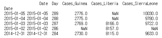
DatetimeIndex에서는 freq 속성이 포함되어 있다.

print(pd.date_range('2017-01-01', '2017-01-07', freq='B'))
평일만 포함된 인덱스를 만들었다.
시간 범위 수정 & 데이터 밀어내기 - shift
만약 나라별로 에볼라의 확산 속도를 비교하려면 발생하기 시작한 날짜를 옮기는 것이 좋다.
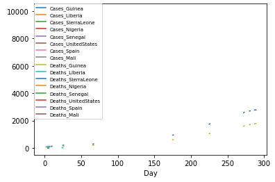
ebola 데이터프레임으로 그래프를 그려보고 에볼라의 확산 속도를 비교하는 데 어떤 문제가 있는지 보자.
import matplotlib.pyplot as plt

ebola.index = ebola['Date']
fig, ax = plt.subplots()
ax = ebola.iloc[0:, 1:].plot(ax=ax)
ax.legend(fontsize=7, loc=2, borderaxespad=0.)
plt.show()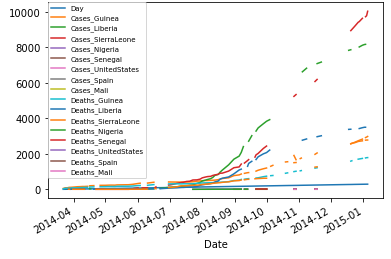
각 나라의 에볼라 발병일이 달라 그래프가 그려지기 시작한 지점이 다르다. 속도를 비교하려면 출발지점을 일치시켜야 한다.
ebola_sub = ebola[['Day', 'Cases_Guinea', 'Cases_Liberia']]
print(ebola_sub.tail(10))
ebola = pd.read_csv('../data/country_timeseries.csv', parse_dates=['Date'])
print(ebola.head().iloc[:, :5])
중간에 누락된 데이터도 포함되어 있다.(2015.01.01)
ebola.index = ebola['Date']
new_idx = pd.date_range(ebola.index.min(), ebola.index.max())
print(new_idx)
idx는 시간 순서가 반대로 되어있다. 이를 반대로 돌리고 새로운 인덱스로 지정하자.
new_idx = reversed(new_idx)
ebola = ebola.reindex(new_idx)
print(ebola.head().iloc[:, :5])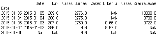
last_valid_index, first_valid_index 메서드를 사용하여 각 나라의 에볼라 발병일을 구해보자.
last_valid = ebola.apply(pd.Series.last_valid_index)
print(last_valid)
print()
first_valid = ebola.apply(pd.Series.first_valid_index)
print(first_valid)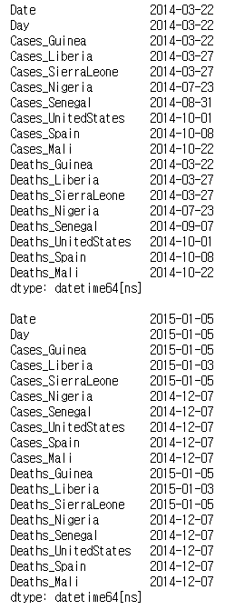
각 나라의 에볼라 발병일을 동일하게 옮기려면 에볼라가 가장 처음 발병한 날에서 각 나라의 에볼라 발병일을 뺀 만큼만 옮기면 된다.
earliest_date = ebola.index.min()
print(earliest_date)
shift_values = last_valid - earliest_date
print(shift_values)
ebola_dict ={}
for idx, col in enumerate(ebola):
    d = shift_values[idx].days
    shifted = ebola[col].shift(d)
ebola_dict[col] = shiftedebola_shift = pd.DataFrame(ebola_dict)print(ebola_shift.tail())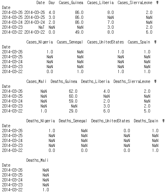
마지막으로 인덱스를 Day 열로 지정하고 그래프에 필요 없는 열을 삭제하면 준비가 끝난다.
ebola_shift.index = ebola_shift['Day']
ebola_shift = ebola_shift.drop(['Date', 'Day'], axis=1)
print(ebola_shift.tail())
fig, ax = plt.subplots()
ax = ebola_shift.iloc[:, :].plot(ax=ax)
ax.legend(fontsize=7, loc=2, borderaxespad=0.)
plt.show()